Life: A Cosmic Fluke or a Common Spark?

One of the most fundamental questions in astrobiology is whether life is common in the universe. The Earth provides an encouraging clue: fossil evidence suggests that life began relatively quickly after our planet became habitable. A naïve interpretation of this fact is that abiogenesis, the origin of life from non-living chemistry, is easy and should occur rapidly wherever conditions are right. Yet this reasoning runs into a major complication: the emergence of intelligent observers like us took almost the entire span of Earth’s habitable history. If intelligence is slow, then life had to begin early on Earth, otherwise we would not exist at all. This selection effect makes early life a weak indicator of rapid abiogenesis unless intelligence is modeled explicitly alongside it.

The paper we are exploring here takes this challenge seriously by developing an objective Bayesian framework that models both life and intelligence as stochastic processes. Unlike earlier analyses, it does not fix the evolutionary timescale from life to intelligence in advance. Instead, both rates are treated as unknowns to be inferred from Earth’s chronology. The key finding is striking: life seems to emerge rapidly, but intelligence is probably rare. This distinction has profound consequences for the Drake Equation and for understanding the “Great Silence” of the universe.

Life and Intelligence as Poisson Processes

The starting point of the analysis is to model abiogenesis and intelligence as Poisson processes. The probability that life emerges by time t_L is given by an exponential distribution:

where \(\lambda_L\) is the abiogenesis rate, measured in events per billion years (Gyr^-1). An identical expression applies for intelligence:

Here, t_I is the time from the appearance of life to the rise of intelligent observers, with \(\lambda_I\) being the rate of intelligence emergence. Both timescales are constrained by the requirement that:

where T is the total habitable window of the planet.

On Earth, this window is estimated as 5.304 Gyr. The planet became stably habitable about 4.404 Gyr ago, and current models predict it will remain habitable for about another 0.9 Gyr. Within this window, the first evidence of life is seen very early. The “optimistic” interpretation uses isotope evidence at 4.1 Gyr ago, which corresponds to t′_L = 0.304 Gyr after habitability began. A more conservative interpretation uses microbial fossils at 3.465 Gyr ago, or t′_L = 0.939 Gyr. In either case, intelligence is observed today, meaning t′_I = 4.404 − t′_L. These numbers set the observational anchors for the Bayesian inference.

Observational Constraints and Piecewise Likelihood Behavior

It is not enough to simply write down the Poisson distributions. The model must be conditioned on what we actually observe: life must have appeared before the first fossil evidence, intelligence must have arisen before today, and both must have fit within the habitable window T. These conditions carve out a region of allowed parameter space. Geometrically, the region looks like a rectangle defined by t_L < t′_L and t_I < t′_I, but truncated by the diagonal t_L + t_I < T.

This setup leads to a piecewise likelihood function, depending on whether the diagonal truncates the rectangle. The condition is:

• Case 1: The allowed region is large, and both early and late life scenarios fit.
• Case 2: The diagonal cuts through the region, and late life scenarios are heavily constrained.

For Earth, substituting values shows that Case 1 applies when t′_L < 0.904 Gyr. With the optimistic evidence (t′_L = 0.304 Gyr), Earth is comfortably in Case 1. With the conservative evidence (t′_L = 0.939 Gyr), we sit right on the boundary.

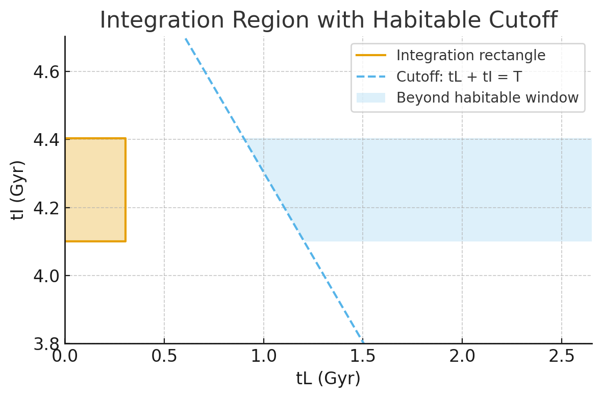
Figure 1A: Optimistic case. The cutoff line lies outside the rectangle, so late-life scenarios remain possible.

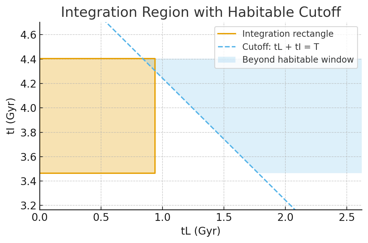
Figure 1B: Conservative case. The cutoff line slices through the rectangle, eliminating part of the integration region.

The Problem of Priors

Bayesian inference requires priors: starting beliefs about the rates \(\lambda_L\) and \(\lambda_I\). Earlier work used power law priors of the form:

But this approach is subjective, since no one knows how to set the cutoffs \(\lambda_{\min}, \lambda_{\max}\). A log uniform prior (n = –1) is often justified as “uninformative,” yet when translated into the more meaningful parameter space of:

—the fraction of worlds where success happens within the habitable window—it introduces hidden biases.

Alternative Priors Beyond Jeffreys

The paper carefully examines n-parameterized priors.

• Haldane prior (n = –1):

This extreme prior heavily weights the boundaries f = 0 and f = 1, meaning it assumes either life is essentially impossible or guaranteed everywhere. However, it is improper: the integral of the distribution diverges, making the posterior non-normalizable.

• Jeffreys prior:

This prior is still tilted toward the extremes, but is softer and proper (normalizable). Transforming back to λ-space gives:

• Uniform prior (n = 0):

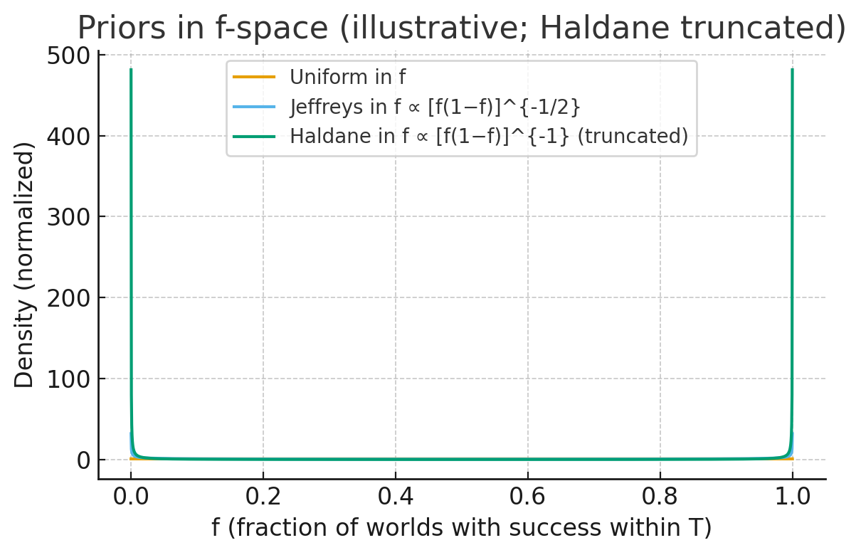
Figure 2: Comparison of priors in f-space. Jeffreys is fair and unbiased, Uniform is flat, Haldane is extreme and improper.

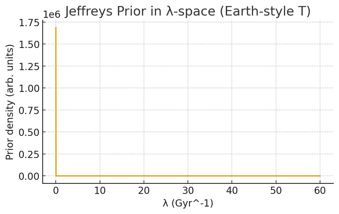
Figure 3: Jeffreys prior in λ-space. It has semi-infinite support and avoids arbitrary cutoffs.

The authors argue that the Jeffreys prior is the most appropriate: it is fair, unbiased, and mathematically wellbehaved. But by also testing uniform and Haldane like priors, they show that the results are not an artifact of prior choice.

Comparing Fast vs. Slow Scenarios

With likelihoods and priors defined, the next step is Bayesian model comparison. The author defines four corner models based on whether life and intelligence are “fast” (λ > 1/t′) or “slow” (λ < 1/t′): M00 (slow life, slow intelligence), M01 (slow life, fast intelligence), M10 (fast life, slow intelligence), and M11 (fast life, fast intelligence).

The evidence shows that fast-intelligence models (M01, M11) are ruled out: they predict civilizations should appear much sooner than they did on Earth. That leaves M00 and M10, which differ only on whether life is fast or slow. The Bayes factor between them comes out to 8.73 in the optimistic fossil case and 2.83 in the conservative case. This means that, conditioned on intelligence being slow, rapid abiogenesis is favored by odds of about 9:1 or 3:1 depending on which fossil evidence you trust.

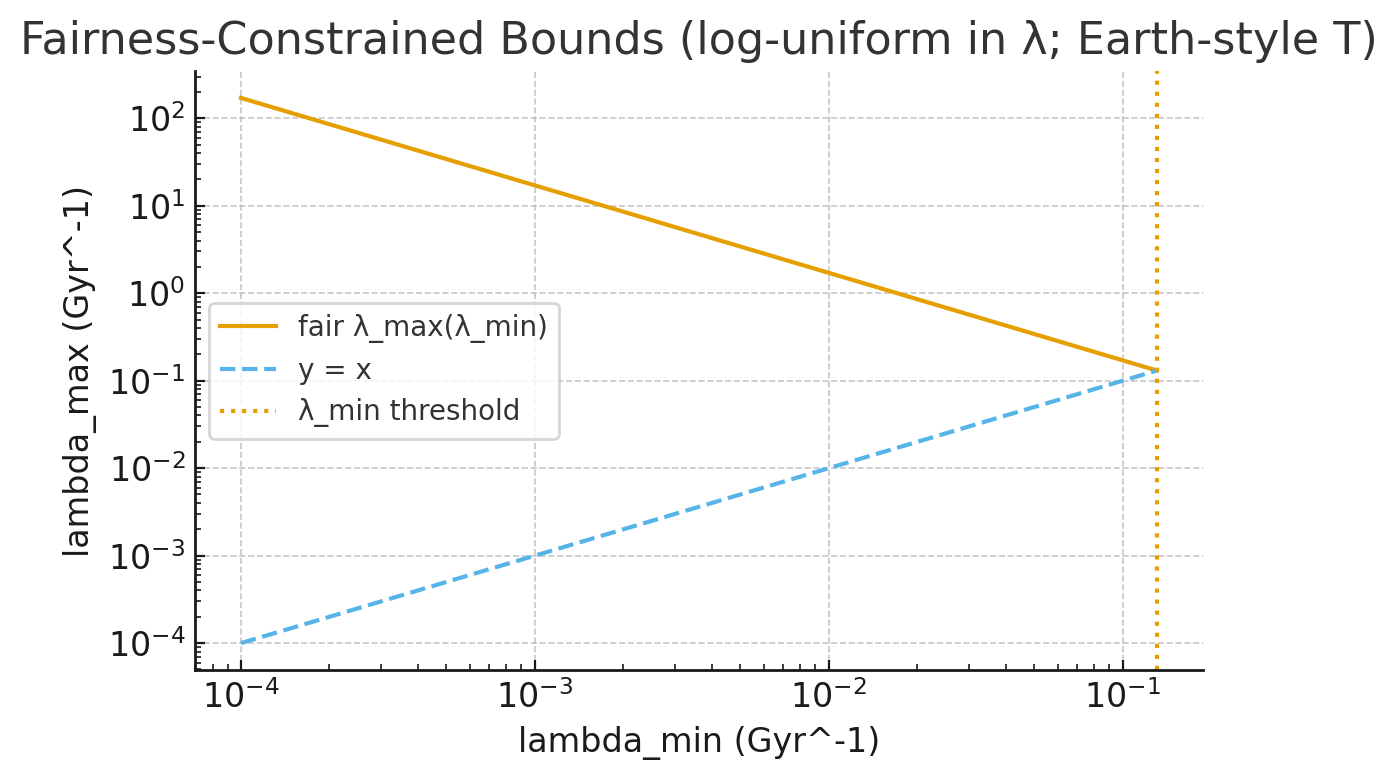
Figure 4: Fairness constraint on λ_min and λ_max under a log-uniform prior. Smaller λ_min forces larger λ_max.

Posterior Distributions

The analysis is reinforced by posterior distributions. When the posteriors are marginalized over the priors and plotted against f_L, the density near f_L → 0 falls below the prior while density near f_L → 1 rises above it. In plain terms, the data actively push probability mass toward “life emerges quickly.”

For intelligence, the picture is weaker. Comparing slow intelligence to the ensemble of all possibilities yields Bayes factors of about 1.5, corresponding to odds of only 3:2. This is a modest tilt toward rarity, but far from conclusive.

Earth-Based Numbers

To ground this in actual numbers: using Earth’s habitable window T = 5.304 Gyr and the optimistic life evidence t′_L = 0.304 Gyr, the Bayes factor for rapid life is nearly 9.5. With the conservative evidence t′_L = 0.939 Gyr, it is just over 3. In both cases, the conclusion is robust to whether one uses Jeffreys or uniform priors. For intelligence, the odds stay close to unity—only a weak preference for slow emergence.

Implications for the Drake Equation and the Great Silence

These results map neatly onto the Drake Equation, which contains a term for the probability of life arising on a habitable planet (f_L) and a term for the probability of intelligence evolving (f_I). The Bayesian framework indicates that f_L is high—life usually starts quickly—but f_I is low or uncertain.

This dual finding resolves a tension in the Fermi Paradox. If microbial life is easy but intelligence is rare, then the galaxy could be teeming with biospheres while still being quiet of civilizations. The Great Silence is not because life is rare, but because intelligence takes too long to evolve and may rarely reach the technological stage.

In plain words: microbes everywhere, people almost nowhere.

Final Thoughts

The strength of this paper lies in its objectivity. By abandoning arbitrary power-law priors in λ-space and adopting the Jeffreys prior in f-space, it eliminates hidden biases. It also treats intelligence as a free parameter rather than a fixed assumption, making the inference more realistic. The conclusion—that life likely begins quickly while intelligence remains rare—provides a Bayesian perspective on the Great Silence that is consistent with both Earth’s fossil record and the absence of other civilizations in our skies.

If we could rerun Earth’s history, life would almost certainly appear again, but whether intelligent observers would emerge is far less certain. That is the true Bayesian lesson of our lonely planet.